Spatial Transcriptomics: Assigning Cell Types in Tissue

Jonathan Alles

EVOBYTE Digital Biology

By EVOBYTE Your partner in bioinformatics

Introduction

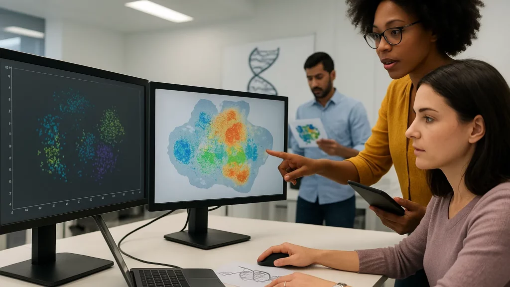
If you’ve ever stared at a spatial transcriptomics heatmap and thought “one dot equals one cell,” you’re not alone. It’s an easy assumption to make, especially when the tissue image looks crisp and the spots line up neatly on top. But in sequencing-based spatial transcriptomics (often shortened to spatial RNA-seq or simply ST), most platforms capture transcripts from areas larger than a single cell. That means each spot often blends signal from multiple neighbors. The result is powerful yet tricky: gene expression measured per spot is usually a mixture.

In this guide, we’ll unpack what a spot really captures, why expression gets mixed, and how that affects downstream analysis. We’ll walk through practical ways to assign spots to cell types and tissue regions, show how single-cell RNA-seq (scRNA-seq) can rescue resolution, and outline the current state of methods you can trust today. Along the way, we’ll share compact code examples and pointers for finding tissue-matched single-cell references, including in the Human Cell Atlas.

What a “spot” really captures in sequencing-based spatial assays

Spatial transcriptomics platforms differ in chemistry and resolution, and that alone shapes how you interpret spots. On 10x Genomics Visium, the capture area is roughly 55 µm in diameter, which typically encompasses clusters of cells rather than a single one. Empirical analyses estimate a median of around 20 cells per Visium spot across certain tissues. Earlier Spatial Transcriptomics (ST) arrays used even larger 100 µm spots, further increasing the chance of mixing. These design choices are not flaws; they’re trade-offs that make whole-transcriptome spatial assays practical at scale. Still, they mean a spot is better viewed as a pixel of tissue than a cell.

The field has raced to push the resolution boundary. Slide-seqV2 uses barcoded beads and achieves approximately 10 µm resolution—near single-cell at the soma level in many tissues—while significantly improving capture efficiency over the original Slide-seq. This shrinks the partial-volume problem but does not eliminate it, especially in tightly packed or layered tissues.

At the other end of the spectrum, platforms like Visium HD now tessellate the capture area into micrometer-scale bins, allowing flexible “binning” up or down to tune sensitivity and resolution for a given sample and sequencing depth. This is a big step toward resolving fine structures while maintaining whole-transcriptome coverage.

The bottom line is simple: a spatial “spot” usually measures a neighborhood, not a single cell. Accept that early, and your analysis will be more realistic from the start.

Why expression per spot is a mixture—and why that matters

Think of each spot as a weighted average of nearby cell types. The weights depend on how much of each cell’s cytoplasm falls inside the capture area, the tissue’s three-dimensional thickness, and technical effects like local RNA diffusion or permeabilization. In layered structures—say, cortex or intestinal villi—adjacent compartments bleed into one another at spot boundaries. When you compute differential expression on raw spot counts, you’re often testing differences in cellular composition more than true per-cell regulation.

This mixing can lead to familiar pitfalls. A marker that appears “expressed in tumor stroma” may actually reflect tumor cells spilling into stromal spots. Conversely, rare cell states can disappear if they’re consistently diluted. Noise compounds when tissue heterogeneity aligns with histology—for example, at the tumor–immune interface—making naïve clustering look more confident than it should be.

You can mitigate these artifacts by explicitly modeling mixtures. Deconvolution methods treat spot counts as sums of cell-type–specific profiles, weighted by cell-type proportions. When you recover those proportions, you convert a blurry image into a layered one, separating “who is where” from “how much of whom.” Benchmarks that compare many methods across tissues consistently show that well-calibrated, reference-based approaches perform strongly for cell-type proportion estimation.

From spots to cell types: deconvolution, label transfer, and gene recovery

There are two common tasks when assigning cell identity in ST data. The first is deconvolution: inferring the proportion of each cell type per spot. The second is label transfer: assigning the most likely label to a spot (or subspot) by aligning it with a reference atlas.

For deconvolution, methods like RCTD, cell2location, DestVI, Stereoscope, SPOTlight, SpatialDWLS, and others use scRNA-seq as a reference to estimate cell-type mixes per spot. Comparative studies report that several of these methods—commonly including cell2location, SpatialDWLS, and RCTD—perform well across diverse datasets. Selecting among them often comes down to your goals (fast and simple vs. Bayesian uncertainty), your compute budget, and whether you want hierarchical or fine-grained cell types.

For label transfer and expression recovery, alignment-based approaches such as Tangram project single cells into tissue space to predict unmeasured genes and sharpen assignments. The advantage is intuitive: if your spatial assay misses lowly expressed genes, a high-quality single-cell atlas can fill the gaps and restore expression patterns that match known biology. Used carefully, this improves downstream analyses like pathway scoring or ligand–receptor inference, especially in sparse data.

Resolution enhancement also helps. BayesSpace “subspots” Visium data, splitting each spot into several smaller units and re-clustering with a spatial prior. This increases effective resolution and sharpens boundaries—useful when cell types change over tens of micrometers rather than hundreds.

Here’s a lightweight example that shows how analysts often connect a Visium dataset with an scRNA-seq reference using R and RCTD via Seurat. This is not meant to be a full pipeline, just a sketch to show the flow.

# R: deconvolve Visium spots with an scRNA-seq reference using RCTD
library(Seurat)
library(spacexr)   # implements RCTD

# spatial: Seurat object with Visium counts and spot coordinates
# sc_ref:  Seurat object with annotated scRNA-seq reference (celltype labels in meta.data)

# prepare RCTD inputs
ref_counts <- GetAssayData(sc_ref, slot = "counts")
cell_types <- sc_ref$celltype
reference  <- Reference(ref_counts, cell_types)

sp_counts  <- GetAssayData(spatial, slot = "counts")
coords     <- GetTissueCoordinates(spatial)
spatialRNA <- SpatialRNA(sp_counts, coords)

# run RCTD (doublet mode handles multi-cell spots)
my_rctd <- create.RCTD(spatialRNA, reference, max_cores = 8, CELL_MIN_INSTANCE = 10)
my_rctd <- run.RCTD(my_rctd, doublet_mode = "doublet")
props   <- my_rctd@results$weights # cell-type proportions per spot

A different but complementary path is to predict gene expression and labels in Python using alignment-based tools. While implementations vary, the conceptual loop is the same: learn a mapping from single-cell to tissue space, project, and then evaluate uncertainty before acting on the results.

Assigning tissue regions: let structure guide identity

Cell types rarely scatter at random. They live in neighborhoods defined by anatomy: cortical layers, tumor–stroma borders, germinal centers, crypt–villus axes. That’s a gift for modeling. Spatial domain methods integrate spot adjacency, gene expression, and sometimes histology to partition tissue into coherent regions. Tools like BayesSpace sharpen Visium grids by splitting spots into subspots, while graph neural network approaches such as SpaGCN incorporate H&E context to better follow histological boundaries. These strategies often cleanly recover layer-like structures and can stabilize downstream deconvolution by providing region-aware priors.

In practice, analysts iterate. They cluster spots into regions, run deconvolution within regions to respect local composition, then refine regions based on updated maps. The loop stops when expression boundaries, histology, and known markers agree. When they don’t, the disagreement is a signal: revisiting QC, segmentation, or the choice of single-cell reference usually resolves it.

How to find single-cell references that actually match your tissue

Reference quality drives deconvolution quality. The most common failure mode is a mismatch between your tissue slice and the scRNA-seq reference. Differences in species, dissociation protocol, disease state, or developmental stage can shift expression programs enough to confuse assignment. Choosing a reference is therefore a data task, not just a citation.

The Human Cell Atlas (HCA) Data Portal is a reliable starting point. It hosts large, standardized single-cell datasets across many tissues, with growing coverage of healthy and disease states and convenient cloud access. When you find candidate references, look closely at metadata fields like tissue, region, processing, and donor characteristics to judge compatibility with your section.

You can also pull ready-to-use references from the CELL×GENE ecosystem. CELLxGENE Discover provides curated datasets with harmonized metadata, and the Census API lets you programmatically filter by tissue, assay, and species, then download single-cell matrices directly. That makes it straightforward to assemble a tissue-matched reference panel for deconvolution or alignment.

Here’s a short Python snippet that illustrates how to query Census for human cells from a given tissue and materialize a reference matrix you can feed into your favorite deconvolution tool.

# Python: fetch a tissue-matched single-cell reference from CELLxGENE Census
import cellxgene_census
import pandas as pd

with cellxgene_census.open_soma(census_version="2025-01-30") as census:
    ad = cellxgene_census.get_anndata(
        census=census,
        organism="Homo sapiens",
        obs_value_filter='tissue_general == "lung" and disease == "normal"',
        var_value_filter='feature_is_filtered == False',
        X_name="raw"
    )

# ad.X is a sparse counts matrix; ad.obs has cell metadata with cell type labels if provided
# Save or subset by cell type as needed for deconvolution/alignment
ad.write_h5ad("lung_reference.h5ad")

If you can’t find a perfect atlas, combine several close ones and harmonize labels. Many methods tolerate moderate label granularity; the crucial part is covering the major compartments present in your tissue. When a rare cell type is missing, keep an eye on residuals or uncertainty scores—well-designed tools will surface that as “unexplained” rather than forcing a wrong label.

Putting it together: a practical mental model

A helpful way to reason about spatial data is to separate three layers of truth. The first layer is composition: which cell types live in each neighborhood and in what proportions. The second is abundance: how many molecules you detected from each type after technical effects. The third is regulation: what genes change within a cell type across regions or conditions.

Sequencing-based spatial assays give you composition and abundance mixed together. Deconvolution recovers composition. Region-aware modeling sharpens boundaries so composition varies smoothly where biology suggests it should. Alignment with single-cell data recovers unmeasured genes and stabilizes label transfer. Once you have a good map of “who is where,” you can finally ask meaningful questions about regulation within types—without being tricked by mixture.

It’s also worth acknowledging the upside of mixture. When spots capture multiple cell types, they carry information about colocalization and potential interactions. Deconvolution followed by neighborhood analysis can reveal where fibroblasts meet T cells, or where specific endothelial subtypes align with smooth muscle. With higher-resolution platforms—like Slide-seqV2 or Visium HD—you can then zoom in to test those hypotheses at finer scales.

Summary / Takeaways

Spatial transcriptomics is a pixelated view of biology. Spots are neighborhoods, not cells, so gene expression per spot is usually a mixture. That simple truth explains a lot of analysis quirks and points you toward the right tools. Use deconvolution to estimate cell-type proportions per spot and label transfer or alignment to project single-cell knowledge into space. Let histology and neighborhood structure guide region calls, and lean on resolution enhancement when boundaries are tight. Most importantly, invest time in selecting a tissue-matched single-cell reference—resources like the Human Cell Atlas and CELL×GENE Census make this practical and reproducible.

If you’re starting a new project, try this thread: pick a high-quality, tissue-matched scRNA-seq reference; run a trusted deconvolution method; refine regions with spatial priors; and only then test within–cell-type changes. You’ll spend less time chasing artifacts and more time discovering biology.