Spatial Omics in Tissue Engineering and Synthetic Biology

Jonathan Alles

EVOBYTE Digital Biology

By EVOBYTE Your partner in bioinformatics

Introduction

If you’ve ever tried to grow a tissue model, you know the sting of unpredictability. Two labs follow the same protocol; only one gets vascularized organoids. A small change in hydrogel stiffness or morphogen timing, and differentiation veers off course. These outcomes aren’t random; they’re spatial. Cells read gradients, respond to neighbors, and sense forces. Yet most assays average signals across space, hiding the very patterns that drive fate decisions.

Spatial omics flips that script. By measuring transcripts, proteins, and even chromatin in situ, it lets us map what our protocols actually paint across a tissue—gradients, niches, and micro-architectures—instead of guessing from bulk means. With that map, bioengineers and synthetic biologists can debug protocols, compare synthetic constructs to native tissue, and move from “it worked in one batch” to designs that are genuinely predictable. Recent reviews and benchmarks show the field has matured rapidly, with technologies and analysis methods now practical for routine engineering workflows.

Why tissue engineering outcomes are so hard to predict

Tissue engineering is a choreography of cues. Cells integrate biochemical morphogens like WNT and BMP, local mechanics from the scaffold, oxygen and nutrient diffusion, and paracrine signals from neighbors. Small shifts in any of these inputs generate different local contexts, and those contexts ripple into different cell fates. That’s why two organoids from the same iPSC line can diverge: early variations in tissue architecture subtly reshape gradients and forces, which then amplify over time.

Even when protocols are harmonized across sites, labs still see divergence in size, metabolism, or long-term differentiation trajectories. It isn’t necessarily “noise”; it’s the microenvironment doing what it does—coupling biology and physics. Controlling fluid dynamics, initial aggregate size, and early morphogenesis can improve reproducibility, precisely because these factors shape spatial context.

Traditional single-cell RNA-seq (scRNA-seq) helps, but it breaks tissues apart, losing the geometry that cells experienced. Imaging helps too, but standard immunofluorescence cannot capture the high-dimensional state space cells occupy. We’ve needed a way to keep the map and the measurements together.

Why spatial transcriptomics changes the game

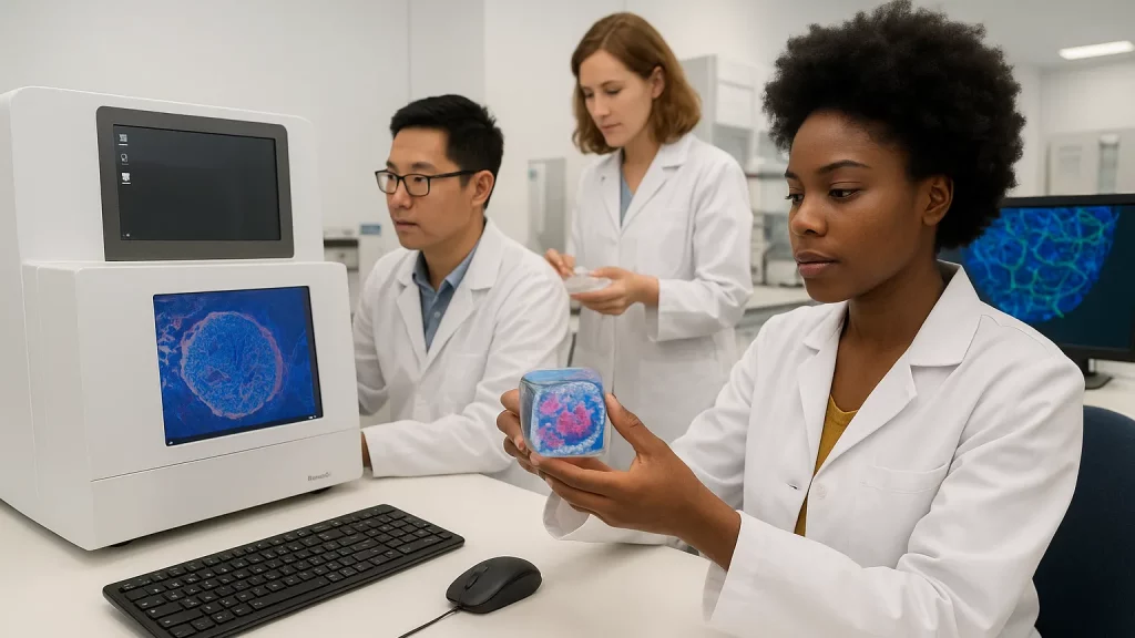
Spatial omics is the umbrella term for molecular assays that preserve location while reading out biology. Two broad families make this possible. Imaging-based methods, like MERFISH or in situ sequencing, visualize hundreds to thousands of RNAs or proteins directly in the tissue. Sequencing-based methods, such as bead or spot–capture platforms, record whole-transcriptome profiles at defined spatial coordinates, often paired with histology. Newer platforms add subcellular resolution or combine modalities, letting you layer transcripts, proteins, and epigenomic marks on the same slide.

For engineering, the payoff is immediate. You can see whether a WNT gradient was steep or shallow, whether endothelial precursors clustered around a scaffold pore, or whether a synthetic circuit induced a ring of Notch activation only at a boundary. Reviews now chart these technologies, their strengths, and where to deploy them. Benchmarks map out performance differences and analysis pitfalls—like when to deconvolve mixed spots and how to cluster spatial domains robustly—so teams can choose methods with eyes open.

Because spatial data lives on a tissue grid, analysis borrows heavily from graph methods. You’ll compute spatial neighbors, detect spatially variable genes, and infer cell–cell communication in physical neighborhoods rather than abstract clusters. That shift—from clusters to coordinates—turns “did differentiation happen?” into “where did differentiation happen, and what local conditions made it happen?”

Mapping engineering outcomes in organoids with spatial biology

Consider a neural organoid protocol where a microfluidic tweak alters media flow. In bulk or dissociated assays, you might spot changes in lineage proportions. With spatial omics, you can go a step further: quantify whether dorsal–ventral patterning bands sharpened, measure how far SHH or WNT targets extend, and test if progenitor zones now sit next to specific stromal or vascular-like niches. Spatial maps also reveal failure modes. If cardiomyocyte clusters form but never couple, you can check whether gap junction genes colocalize with the beating regions or remain marooned behind a stiffness mismatch in the matrix.

This is not speculative. Studies are creating integrated organoid atlases that reveal how differentiation trajectories and tissue architectures emerge. Others show that controlling early physical conditions—like fluid dynamics during morphogenesis—reduces variability by shaping spatial organization from the start. Together, these insights show why protocol changes impact outcomes: they redraw the landscape cells read.

Spatial omics also helps when engineering synthetic organizers or patterning circuits. By mapping morphogen induction domains and downstream gene programs in situ, you can verify that a designed WNT source produced the intended gradient and that the gradient translated into the desired anterior–posterior fate map. You can even ask whether alternative circuit topologies produce comparable spatial outputs or steer the system into a different morphospace entirely.

How to compare synthetic constructs to real tissue with spatial omics

When you claim fidelity—“our liver construct behaves like adult liver”—the key question is: like which region, at what developmental stage, and in what microenvironment? Spatial omics lets you answer with evidence, not metaphors.

One practical approach starts with a reference atlas of primary tissue. You align organoid or engineered-tissue maps to the atlas, compare spatially variable programs, and quantify how well domains match. You don’t just match cell types; you compare neighborhood compositions and ligand–receptor circuits that define niches. Recent organoid atlases formalize this comparison by projecting engineered cells onto fetal and adult references and reporting on-target versus off-target states. With spatial data, you can extend this idea to matching tissue domains, not just cell identities, and to measuring how far engineered domains deviate in space and signaling.

Benchmarks of imaging-based and sequencing-based platforms show meaningful differences in sensitivity, resolution, and throughput, so pick the platform that matches your fidelity question. If you care about subcellular localization or fine tissue boundaries, single-cell imaging platforms help. If you need unbiased, whole-transcriptome views over large areas, spatial capture approaches shine. Analysis benchmarks also clarify which clustering and domain-calling methods are most robust across tissues, making your fidelity metrics more defensible.

Here’s a compact example of how you might operationalize fidelity with open tools. Suppose you have a spatial organoid dataset and a spatial atlas of native tissue. You can align cell states, compare spatially variable programs, and compute a fidelity score for each region.

Sometimes your spatial data has multi-cell capture spots. In those cases, deconvolution becomes essential. Robust methods estimate the cell-type mixture within each spot, making downstream comparisons fairer. Recent surveys and reviews provide guidance on when to deconvolve and how to validate that step for engineering use cases.

A practical path from protocol to spatial insight

You don’t need to spatially profile every sample to benefit. A strategic cadence works well. Use standard scRNA-seq during rapid iteration to screen conditions. At decision points—new scaffold, altered morphogen schedule, or circuit redesign—collect spatial datasets to check whether the protocol draws the intended map. The return on that investment is confidence: you can quantify whether a new step created the gradient, boundary, or niche you were aiming for.

Start by deciding the spatial scale that matters to your question. If you are engineering vascular ingress, you need neighborhood-scale resolution and good endothelial markers. If you are testing a morphogen circuit, prioritize whole-slide coverage to capture gradients end to end. Technology comparisons across tumor and FFPE samples generalize surprisingly well to development and organoids: they’ll help you choose between imaging-based single-cell platforms and capture-based approaches depending on whether resolution or unbiased discovery is paramount.

On the analysis side, lean on established benchmarks. Choose clustering and domain-calling methods that perform consistently across datasets. Favor transparent, reproducible pipelines, and plan for data integration with histology. Many teams now align image features and spatial gene expression to reduce costs and extend insights, aided by well-tested frameworks for multimodal integration. These approaches won’t replace wet-lab spatial assays for engineering decisions, but they can stretch your budget and strengthen conclusions between experimental checkpoints.

When your aim is reproducibility, pay special attention to early-stage architecture. Controlled fluid dynamics, aggregate size standardization, and scaffold mechanics shape the spatial canvas on which your protocols act. Spatial readouts then verify that your controls did what you intended: produced consistent domain sizes, preserved boundary sharpness, or stabilized niche composition across batches and sites. That pairing—physical control plus spatial verification—has started to reduce batch-to-batch drift in organoid models.

Summary / Takeaways

Spatial omics gives bioengineers and synthetic biologists something we’ve lacked: a faithful map of what our protocols actually impose across a tissue. Because cells decide fate locally, that map is the difference between a design that’s merely plausible and a design that is predictable.

Use spatial omics to see how protocol changes redraw gradients, niches, and boundaries. Align engineered maps to native-tissue atlases, and report fidelity as spatial metrics rather than anecdotes. Choose platforms and analysis methods that match your design question, guided by technology and method benchmarks. And couple spatial readouts with physical controls—of fluid dynamics, scaffold mechanics, and early architecture—to convert fragile protocols into robust ones.

The big shift is cultural as much as technical. Instead of asking only “which cell types did we get?”, we now ask “where did they arise, what local rules put them there, and how closely does that match the tissue we’re emulating?” Answer those questions well, and the path from synthetic plan to living tissue becomes far less mysterious.